
The data set used in this demo is an email marketing campaign data that includes customer information, described below, as a well as whether the customer responded to the marketing campaign or not. The machine learning task is to design a model that will be able to predict whether a customer will respond to the marketing campaign based on his/her information. In other words, predict the ‘responded’ target variable described in the data based on all the input variables provided.
1- Data Preparation
import pandas as pd
    # Data is avavilable in https://github.com/mohcinemadkour/github-open-data-portal
data = pd.read_csv('marketing_training.csv')
test = pd.read_csv('marketing_test.csv')
data.shape
(7414, 22)

data['responded'] = data['responded'].map({'no': 0, 'yes': 1})

X_data = data.iloc[:, 0:21]
y_data = data.iloc[:, 21:22]
Data Engineering (pmonths and pdays)
For columns pmonths and pdays we have a symbol value (999) which means that client was not previuously contacted. As preprocessing of this info we are going to create an additional column called was_not_previously_contacted that represent the fact that either the client was contacted or not
# Make sure of the consistency of 999 over pmonths and pdays
(X_data[X_data["pmonths"]==999]).equals(X_data[X_data["pdays"]==999])

True


import numpy as np
X_data["was_not_previously_contacted"] = np.where(X_data["pmonths"]==999,1,0)
Missing values analysis
def missing_values_table(df):
    """Calculate missing values by column, tabulate results

    Input
    df: The dataframe
    """
    # Total missing values
    mis_val = df.isnull().sum()

    # Percentage of missing values
    mis_val_percent = 100 * df.isnull().sum() / len(df)

    # Make a table with the results
    mis_val_table = pd.concat([mis_val, mis_val_percent], axis=1)

    # Rename the columns
    mis_val_table_ren_columns = mis_val_table.rename(
    columns = {0 : 'Missing Values', 1 : '% of Total Values'})

    # Sort the table by percentage of missing descending
    mis_val_table_ren_columns = mis_val_table_ren_columns[
        mis_val_table_ren_columns.iloc[:,1] != 0].sort_values(
    '% of Total Values', ascending=False).round(1)

    # Print some summary information
    print ("Your selected dataframe has " + str(df.shape[1]) + " columns.\n"
        "There are " + str(mis_val_table_ren_columns.shape[0]) +
          " columns that have missing values.")

    # Return the dataframe with missing information
    return mis_val_table_ren_columns
missing_values_table(X_data)
Your selected dataframe has 22 columns.
There are 3 columns that have missing values.
| Missing Values | % of Total Values | |
|---|---|---|
| schooling | 2155 | 29.1 |
| custAge | 1804 | 24.3 |
| day_of_week | 711 | 9.6 |
#!pip install missingno
import missingno as msno
msno.matrix(X_data)
<matplotlib.axes._subplots.AxesSubplot at 0x7f782f264650>
I can see that: - custAge column has missing values with variation in occurrence, - schooling column are almost filled with missing values with variation in occurrence, and - day_of_week column has missing values that are sparsely located
From this visualization it is important to know the fact that there is no correlation in missing value locations of the columns with missing values The bar on the right side of this diagram shows the data completeness for each row. In this dataset, all rows have 18 - 21 valid values and hence 0 - 3 missing values.
Also, missingno.heatmap visualizes the correlation matrix about the locations of missing values in columns.
msno.heatmap(X_data)
<matplotlib.axes._subplots.AxesSubplot at 0x7f7844ff71d0>
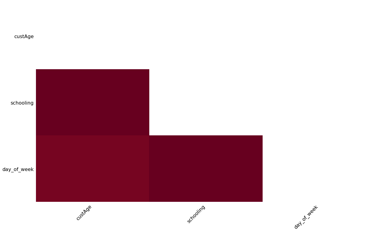
I have missing values in custAge which is a numerical variable, and in schooling and day_of_week which are categorical variables
Missing values removal
KNN (K Nearest Neighbors)
I use a KNN based machine learning technique for data imputation. In this method, k neighbors are chosen based on some distance measure and their average is used as an imputation estimate. The method requires the selection of the number of nearest neighbors, and a distance metric. KNN can predict both discrete attributes (the most frequent value among the k nearest neighbors) and continuous attributes (the mean among the k nearest neighbors) The distance metric varies according to the type of data: 1. Continuous Data: The commonly used distance metrics for continuous data are Euclidean, Manhattan and Cosine 2. Categorical Data: Hamming distance is generally used in this case. It takes all the categorical attributes and for each, count one if the value is not the same between two points. The Hamming distance is then equal to the number of attributes for which the value was different. One of the most attractive features of the KNN algorithm is that it is simple to understand and easy to implement. The non-parametric nature of KNN gives it an edge in certain settings where the data may be highly “unusual”. One of the obvious drawbacks of the KNN algorithm is that it becomes time-consuming when analyzing large datasets because it searches for similar instances through the entire dataset. Furthermore, the accuracy of KNN can be severely degraded with high-dimensional data because there is little difference between the nearest and farthest neighbor.
##### Code and Documentation Credit : https://towardsdatascience.com/the-use-of-knn-for-missing-values-cf33d935c637
https://towardsdatascience.com/how-to-handle-missing-data-8646b18db0d4
https://gist.github.com/YohanObadia/b310793cd22a4427faaadd9c381a5850
import numpy as np
import pandas as pd
from collections import defaultdict
from scipy.stats import hmean
from scipy.spatial.distance import cdist
from scipy import stats
import numbers


def weighted_hamming(data):
    """ Compute weighted hamming distance on categorical variables. For one variable, it is equal to 1 if
        the values between point A and point B are different, else it is equal the relative frequency of the
        distribution of the value across the variable. For multiple variables, the harmonic mean is computed
        up to a constant factor.
        @params:
            - data = a pandas data frame of categorical variables
        @returns:
            - distance_matrix = a distance matrix with pairwise distance for all attributes
    """
    categories_dist = []

    for category in data:
        X = pd.get_dummies(data[category])
        X_mean = X * X.mean()
        X_dot = X_mean.dot(X.transpose())
        X_np = np.asarray(X_dot.replace(0,1,inplace=False))
        categories_dist.append(X_np)
    categories_dist = np.array(categories_dist)
    distances = hmean(categories_dist, axis=0)
    return distances


def distance_matrix(data, numeric_distance = "euclidean", categorical_distance = "jaccard"):
    """ Compute the pairwise distance attribute by attribute in order to account for different variables type:
        - Continuous
        - Categorical
        For ordinal values, provide a numerical representation taking the order into account.
        Categorical variables are transformed into a set of binary ones.
        If both continuous and categorical distance are provided, a Gower-like distance is computed and the numeric
        variables are all normalized in the process.
        If there are missing values, the mean is computed for numerical attributes and the mode for categorical ones.

        Note: If weighted-hamming distance is chosen, the computation time increases a lot since it is not coded in C
        like other distance metrics provided by scipy.
        @params:
            - data                  = pandas dataframe to compute distances on.
            - numeric_distances     = the metric to apply to continuous attributes.
                                      "euclidean" and "cityblock" available.
                                      Default = "euclidean"
            - categorical_distances = the metric to apply to binary attributes.
                                      "jaccard", "hamming", "weighted-hamming" and "euclidean"
                                      available. Default = "jaccard"
        @returns:
            - the distance matrix
    """
    possible_continuous_distances = ["euclidean", "cityblock"]
    possible_binary_distances = ["euclidean", "jaccard", "hamming", "weighted-hamming"]
    number_of_variables = data.shape[1]
    number_of_observations = data.shape[0]

    # Get the type of each attribute (Numeric or categorical)
    is_numeric = [all(isinstance(n, numbers.Number) for n in data.iloc[:, i]) for i, x in enumerate(data)]
    is_all_numeric = sum(is_numeric) == len(is_numeric)
    is_all_categorical = sum(is_numeric) == 0
    is_mixed_type = not is_all_categorical and not is_all_numeric

    # Check the content of the distances parameter
    if numeric_distance not in possible_continuous_distances:
        print "The continuous distance " + numeric_distance + " is not supported."
        return None
    elif categorical_distance not in possible_binary_distances:
        print "The binary distance " + categorical_distance + " is not supported."
        return None

    # Separate the data frame into categorical and numeric attributes and normalize numeric data
    if is_mixed_type:
        number_of_numeric_var = sum(is_numeric)
        number_of_categorical_var = number_of_variables - number_of_numeric_var
        data_numeric = data.iloc[:, is_numeric]
        data_numeric = (data_numeric - data_numeric.mean()) / (data_numeric.max() - data_numeric.min())
        data_categorical = data.iloc[:, [not x for x in is_numeric]]

    # Replace missing values with column mean for numeric values and mode for categorical ones. With the mode, it
    # triggers a warning: "SettingWithCopyWarning: A value is trying to be set on a copy of a slice from a DataFrame"
    # but the value are properly replaced
    if is_mixed_type:
        data_numeric.fillna(data_numeric.mean(), inplace=True)
        for x in data_categorical:
            data_categorical[x].fillna(data_categorical[x].mode()[0], inplace=True)
    elif is_all_numeric:
        data.fillna(data.mean(), inplace=True)
    else:
        for x in data:
            data[x].fillna(data[x].mode()[0], inplace=True)

    # "Dummifies" categorical variables in place
    if not is_all_numeric and not (categorical_distance == 'hamming' or categorical_distance == 'weighted-hamming'):
        if is_mixed_type:
            data_categorical = pd.get_dummies(data_categorical)
        else:
            data = pd.get_dummies(data)
    elif not is_all_numeric and categorical_distance == 'hamming':
        if is_mixed_type:
            data_categorical = pd.DataFrame([pd.factorize(data_categorical[x])[0] for x in data_categorical]).transpose()
        else:
            data = pd.DataFrame([pd.factorize(data[x])[0] for x in data]).transpose()

    if is_all_numeric:
        result_matrix = cdist(data, data, metric=numeric_distance)
    elif is_all_categorical:
        if categorical_distance == "weighted-hamming":
            result_matrix = weighted_hamming(data)
        else:
            result_matrix = cdist(data, data, metric=categorical_distance)
    else:
        result_numeric = cdist(data_numeric, data_numeric, metric=numeric_distance)
        if categorical_distance == "weighted-hamming":
            result_categorical = weighted_hamming(data_categorical)
        else:
            result_categorical = cdist(data_categorical, data_categorical, metric=categorical_distance)
        result_matrix = np.array([[1.0*(result_numeric[i, j] * number_of_numeric_var + result_categorical[i, j] *
                               number_of_categorical_var) / number_of_variables for j in range(number_of_observations)] for i in range(number_of_observations)])

    # Fill the diagonal with NaN values
    np.fill_diagonal(result_matrix, np.nan)

    return pd.DataFrame(result_matrix)


def knn_impute(target, attributes, k_neighbors, aggregation_method="mean", numeric_distance="euclidean",
               categorical_distance="jaccard", missing_neighbors_threshold = 0.5):
    """ Replace the missing values within the target variable based on its k nearest neighbors identified with the
        attributes variables. If more than 50% of its neighbors are also missing values, the value is not modified and
        remains missing. If there is a problem in the parameters provided, returns None.
        If to many neighbors also have missing values, leave the missing value of interest unchanged.
        @params:
            - target                        = a vector of n values with missing values that you want to impute. The length has
                                              to be at least n = 3.
            - attributes                    = a data frame of attributes with n rows to match the target variable
            - k_neighbors                   = the number of neighbors to look at to impute the missing values. It has to be a
                                              value between 1 and n.
            - aggregation_method            = how to aggregate the values from the nearest neighbors (mean, median, mode)
                                              Default = "mean"
            - numeric_distances             = the metric to apply to continuous attributes.
                                              "euclidean" and "cityblock" available.
                                              Default = "euclidean"
            - categorical_distances         = the metric to apply to binary attributes.
                                              "jaccard", "hamming", "weighted-hamming" and "euclidean"
                                              available. Default = "jaccard"
            - missing_neighbors_threshold   = minimum of neighbors among the k ones that are not also missing to infer
                                              the correct value. Default = 0.5
        @returns:
            target_completed        = the vector of target values with missing value replaced. If there is a problem
                                      in the parameters, return None
    """

    # Get useful variables
    possible_aggregation_method = ["mean", "median", "mode"]
    number_observations = len(target)
    is_target_numeric = all(isinstance(n, numbers.Number) for n in target)

    # Check for possible errors
    if number_observations < 3:
        print "Not enough observations."
        return None
    if attributes.shape[0] != number_observations:
        print "The number of observations in the attributes variable is not matching the target variable length."
        return None
    if k_neighbors > number_observations or k_neighbors < 1:
        print "The range of the number of neighbors is incorrect."
        return None
    if aggregation_method not in possible_aggregation_method:
        print "The aggregation method is incorrect."
        return None
    if not is_target_numeric and aggregation_method != "mode":
        print "The only method allowed for categorical target variable is the mode."
        return None

    # Make sure the data are in the right format
    target = pd.DataFrame(target)
    attributes = pd.DataFrame(attributes)

    # Get the distance matrix and check whether no error was triggered when computing it
    distances = distance_matrix(attributes, numeric_distance, categorical_distance)
    if distances is None:
        return None

    # Get the closest points and compute the correct aggregation method
    for i, value in enumerate(target.iloc[:, 0]):
        if pd.isnull(value):
            order = distances.iloc[i,:].values.argsort()[:k_neighbors]
            closest_to_target = target.iloc[order, :]
            missing_neighbors = [x for x  in closest_to_target.isnull().iloc[:, 0]]
            # Compute the right aggregation method if at least more than 50% of the closest neighbors are not missing
            if sum(missing_neighbors) >= missing_neighbors_threshold * k_neighbors:
                continue
            elif aggregation_method == "mean":
                target.iloc[i] = np.ma.mean(np.ma.masked_array(closest_to_target,np.isnan(closest_to_target)))
            elif aggregation_method == "median":
                target.iloc[i] = np.ma.median(np.ma.masked_array(closest_to_target,np.isnan(closest_to_target)))
            else:
                target.iloc[i] = stats.mode(closest_to_target, nan_policy='omit')[0][0]

    return target
I started with k_neighbors = 5 but that keep the data with some missing values, then I start incrementing this parametre until I got 100% of imputation of missing values with k_neighbors= 350
X_data["day_of_week"]=knn_impute(X_data["day_of_week"], X_data, k_neighbors= 350, aggregation_method="mode", numeric_distance="euclidean",
               categorical_distance="jaccard", missing_neighbors_threshold = 0.5)
X_data["schooling"]=knn_impute(X_data["schooling"], X_data, k_neighbors=350, aggregation_method="mode", numeric_distance="euclidean",
               categorical_distance="jaccard", missing_neighbors_threshold = 0.5)
X_data["custAge"]=knn_impute(X_data["custAge"], X_data, k_neighbors=350, aggregation_method="mean", numeric_distance="euclidean",
               categorical_distance="jaccard", missing_neighbors_threshold = 0.5)
Checking if there is any missing values after imputation
import missingno as msno
msno.matrix(X_data)
<matplotlib.axes._subplots.AxesSubplot at 0x7f7854a74c50>
missing_values_table(X_data)
Your selected dataframe has 22 columns.
There are 0 columns that have missing values.
| Missing Values | % of Total Values |
|---|
Numerical data
X_data.info()
<class 'pandas.core.frame.DataFrame'>
RangeIndex: 7414 entries, 0 to 7413
Data columns (total 22 columns):
custAge                         7414 non-null float64
profession                      7414 non-null object
marital                         7414 non-null object
schooling                       7414 non-null object
default                         7414 non-null object
housing                         7414 non-null object
loan                            7414 non-null object
contact                         7414 non-null object
month                           7414 non-null object
day_of_week                     7414 non-null object
campaign                        7414 non-null int64
pdays                           7414 non-null int64
previous                        7414 non-null int64
poutcome                        7414 non-null object
emp.var.rate                    7414 non-null float64
cons.price.idx                  7414 non-null float64
cons.conf.idx                   7414 non-null float64
euribor3m                       7414 non-null float64
nr.employed                     7414 non-null float64
pmonths                         7414 non-null float64
pastEmail                       7414 non-null int64
was_not_previously_contacted    7414 non-null int64
dtypes: float64(7), int64(5), object(10)
memory usage: 1.2+ MB
X_data.describe()
| custAge | campaign | pdays | previous | emp.var.rate | cons.price.idx | cons.conf.idx | euribor3m | nr.employed | pmonths | pastEmail | was_not_previously_contacted | |
|---|---|---|---|---|---|---|---|---|---|---|---|---|
| count | 7414.000000 | 7414.000000 | 7414.000000 | 7414.000000 | 7414.000000 | 7414.000000 | 7414.000000 | 7414.000000 | 7414.000000 | 7414.000000 | 7414.000000 | 7414.000000 |
| mean | 39.723855 | 2.518344 | 960.024548 | 0.184111 | 0.052091 | 93.570708 | -40.561316 | 3.583141 | 5165.224251 | 959.797028 | 0.361883 | 0.960750 |
| std | 9.243954 | 2.695055 | 192.845029 | 0.516775 | 1.568399 | 0.578345 | 4.649800 | 1.744865 | 73.108669 | 193.969418 | 1.261668 | 0.194202 |
| min | 18.000000 | 1.000000 | 0.000000 | 0.000000 | -3.400000 | 92.201000 | -50.800000 | 0.634000 | 4963.600000 | 0.000000 | 0.000000 | 0.000000 |
| 25% | 34.000000 | 1.000000 | 999.000000 | 0.000000 | -1.800000 | 93.075000 | -42.700000 | 1.334000 | 5099.100000 | 999.000000 | 0.000000 | 1.000000 |
| 50% | 38.559547 | 2.000000 | 999.000000 | 0.000000 | 1.100000 | 93.444000 | -41.800000 | 4.857000 | 5191.000000 | 999.000000 | 0.000000 | 1.000000 |
| 75% | 44.000000 | 3.000000 | 999.000000 | 0.000000 | 1.400000 | 93.994000 | -36.400000 | 4.961000 | 5228.100000 | 999.000000 | 0.000000 | 1.000000 |
| max | 94.000000 | 40.000000 | 999.000000 | 6.000000 | 1.400000 | 94.767000 | -26.900000 | 5.045000 | 5228.100000 | 999.000000 | 18.000000 | 1.000000 |
It is worth noting that the min, mean, max and 25%,50%75% are properly ordered, therefore the numerical data looks good and there is no need to cast/coerse to numeric
# Scale numerical features
scaled_num_data = pd.DataFrame(StandardScaler().fit_transform(num_data), columns=num_data.keys())
/home/mohcine/Software/anaconda2/lib/python2.7/site-packages/sklearn/preprocessing/data.py:645: DataConversionWarning: Data with input dtype int64, float64 were all converted to float64 by StandardScaler.
  return self.partial_fit(X, y)
/home/mohcine/Software/anaconda2/lib/python2.7/site-packages/sklearn/base.py:464: DataConversionWarning: Data with input dtype int64, float64 were all converted to float64 by StandardScaler.
  return self.fit(X, **fit_params).transform(X)
Outlier detection and cleaning
fig1 = pd.scatter_matrix(scaled_num_data, alpha = 0.3, figsize = (11,11), diagonal = 'kde')
/home/mohcine/Software/anaconda2/lib/python2.7/site-packages/ipykernel_launcher.py:1: FutureWarning: pandas.scatter_matrix is deprecated, use pandas.plotting.scatter_matrix instead
  """Entry point for launching an IPython kernel.
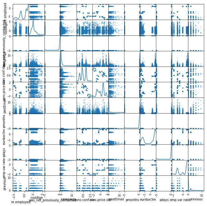
From the scatter plot I dont see bad outliers in the data
One-hot encode the categorical data
# The OneHotEncoder only works on categorical features. We need first to extract the categorial featuers using boolean mask.
# Categorical boolean mask
categorical_feature_mask = X_data.dtypes==object

# filter categorical columns using mask and turn it into a list
categorical_cols = X_data.columns[categorical_feature_mask].tolist()
# find unique labels for each category
X_data[categorical_cols].apply(lambda x: x.nunique(), axis=0)
profession     12
marital         4
schooling       8
default         3
housing         3
loan            3
contact         2
month          10
day_of_week     5
poutcome        3
dtype: int64
Pandas get_dummies method get the dummy variables for categorical features.
# apply One-Hot Encoder on categorical feature columns
cat_data = pd.get_dummies(X_data[categorical_cols])
cat_data.tail(5)
| profession_admin. | profession_blue-collar | profession_entrepreneur | profession_housemaid | profession_management | profession_retired | profession_self-employed | profession_services | profession_student | profession_technician | ... | month_oct | month_sep | day_of_week_fri | day_of_week_mon | day_of_week_thu | day_of_week_tue | day_of_week_wed | poutcome_failure | poutcome_nonexistent | poutcome_success | |
|---|---|---|---|---|---|---|---|---|---|---|---|---|---|---|---|---|---|---|---|---|---|
| 7409 | 0 | 1 | 0 | 0 | 0 | 0 | 0 | 0 | 0 | 0 | ... | 0 | 0 | 0 | 0 | 0 | 0 | 1 | 0 | 1 | 0 |
| 7410 | 0 | 1 | 0 | 0 | 0 | 0 | 0 | 0 | 0 | 0 | ... | 0 | 0 | 0 | 0 | 0 | 1 | 0 | 0 | 1 | 0 |
| 7411 | 0 | 1 | 0 | 0 | 0 | 0 | 0 | 0 | 0 | 0 | ... | 0 | 0 | 1 | 0 | 0 | 0 | 0 | 1 | 0 | 0 |
| 7412 | 0 | 0 | 0 | 0 | 0 | 0 | 0 | 0 | 0 | 0 | ... | 0 | 0 | 0 | 0 | 1 | 0 | 0 | 0 | 1 | 0 |
| 7413 | 0 | 1 | 0 | 0 | 0 | 0 | 0 | 0 | 0 | 0 | ... | 0 | 0 | 1 | 0 | 0 | 0 | 0 | 0 | 1 | 0 |
5 rows × 53 columns
Notice the new categories that were created. For example, the categorical variable "marital" is split into three categories, 'marital_divorced', 'marital_married', 'marital_single', 'marital_unknown'. Now, that the one hot encoding of the categorical data is done, I need to merge the numerical data from the original data.
Concatenation
numerical_cols = list(set(X_data.columns.values.tolist()) - set(categorical_cols))
num_data = X_data[numerical_cols].copy()

# check that the numeric data has been captured accurately
num_data.head()
| nr.employed | custAge | was_not_previously_contacted | campaign | cons.conf.idx | cons.price.idx | pastEmail | pmonths | euribor3m | pdays | emp.var.rate | previous | |
|---|---|---|---|---|---|---|---|---|---|---|---|---|
| 0 | 5195.8 | 55.000000 | 1 | 1 | -42.0 | 93.200 | 0 | 999.0 | 4.191 | 999 | -0.1 | 0 |
| 1 | 5228.1 | 37.673913 | 1 | 1 | -42.7 | 93.918 | 0 | 999.0 | 4.960 | 999 | 1.4 | 0 |
| 2 | 5191.0 | 42.000000 | 1 | 1 | -36.4 | 93.994 | 0 | 999.0 | 4.857 | 999 | 1.1 | 0 |
| 3 | 5228.1 | 55.000000 | 1 | 2 | -42.7 | 93.918 | 0 | 999.0 | 4.962 | 999 | 1.4 | 0 |
| 4 | 5099.1 | 37.251082 | 1 | 5 | -46.2 | 92.893 | 1 | 999.0 | 1.291 | 999 | -1.8 | 1 |
# concat numeric and the encoded categorical variables
num_cat_data = pd.concat([num_data, cat_data], axis=1)

# here we do a quick sanity check that the data has been concatenated correctly by checking the dimension of the vectors
print(cat_data.shape)
print(num_data.shape)
print(num_cat_data.shape)
(7414, 53)
(7414, 12)
(7414, 65)
Spliting to training & testing
Since I dont have the responded vector in the test set (label), I am going to split the training set to train set + test set
from sklearn.model_selection import train_test_split
x_train, x_test, y_train, y_test = train_test_split(num_cat_data,
                                                    y_data,
                                                    test_size=.25,
                                                    random_state=42)
# check that the dimensions of our train and test sets are okay
print(x_train.shape)
print(y_train.shape)
print(x_test.shape)
print(y_test.shape)
(5560, 65)
(5560, 1)
(1854, 65)
(1854, 1)
Pickling
import pickle
# save the datasets for later use
preprocessed_data = {
    'x_train':x_train,
    'y_train':y_train,
    'x_test':x_test,
    'y_test':y_test,
}

# pickle the preprocessed_data
path = 'preprocessed_data_full.pkl'
out = open(path, 'wb')
pickle.dump(preprocessed_data, out)
out.close()
Fix class imbalance
Training a machine learning model on an imbalanced dataset can introduce unique challenges to the learning problem. Imbalanced data typically refers to a classification problem where the number of observations per class is not equally distributed; often you'll have a large amount of data/observations for one class (referred to as the majority class), and much fewer observations for one or more other classes (referred to as the minority classes). It's worth noting that not all datasets are affected equally by class imbalance. Generally, for easy classification problems in which there's a clear separation in the data, class imbalance doesn't impede on the model's ability to learn effectively. However, datasets that are inherently more difficult to learn from see an amplification in the learning challenge when a class imbalance is introduced.
#!pip install imblearn
from imblearn.over_sampling import SMOTE
#Before fitting SMOTE, let us check the y_train values:
y_train['responded'].value_counts()
0    4969
1     591
Name: responded, dtype: int64
591.0/4969.0*100
11.893741195411552
I have only 11% of responded customers, so there’s some imbalance in the data but it’s not very terrible.
Oversampling Minor class using SMOTE algorithm on Training data set Only
I’ll upsample the positive responded using the SMOTE algorithm (Synthetic Minority Oversampling Technique). At a high level, SMOTE creates synthetic observations of the minority class (bad loans) by:
- Finding the k-nearest-neighbors for minority class observations (finding similar observations)
- Randomly choosing one of the k-nearest-neighbors and using it to create a similar, but randomly tweaked, new observation.
After upsampling to a class ratio of 1.0, I should have a balanced dataset.
sm = SMOTE(random_state=12, ratio = 1.0)
x_train, y_train = sm.fit_sample(x_train, y_train)
/home/mohcine/Software/anaconda2/lib/python2.7/site-packages/sklearn/utils/validation.py:761: DataConversionWarning: A column-vector y was passed when a 1d array was expected. Please change the shape of y to (n_samples, ), for example using ravel().
  y = column_or_1d(y, warn=True)
np.bincount(y_train)
array([4969, 4969])
Conclusion
It is worth noticing that by oversampling only on the training data, none of the information in the test data is being used to create synthetic observations. So these results should be generalizable
2- Exploratory Data Analysis
- Numeric features correlation analysis
- Creating a simple baseline model (the parsimonious model)
- Testing the oversampling on training set
- Estimate feature importance by training a random forest regressor
# Run this cell and a very nice matrix will hopefully appear
import matplotlib.pyplot as plt
import numpy as np
import seaborn as sns
fig, ax = plt.subplots(figsize=(12,12))
sns.heatmap(num_data.corr(),annot=True, center=0, cmap='BrBG', annot_kws={"size": 14})
fig.show()
/home/mohcine/Software/anaconda2/lib/python2.7/site-packages/matplotlib/figure.py:457: UserWarning: matplotlib is currently using a non-GUI backend, so cannot show the figure
  "matplotlib is currently using a non-GUI backend, "
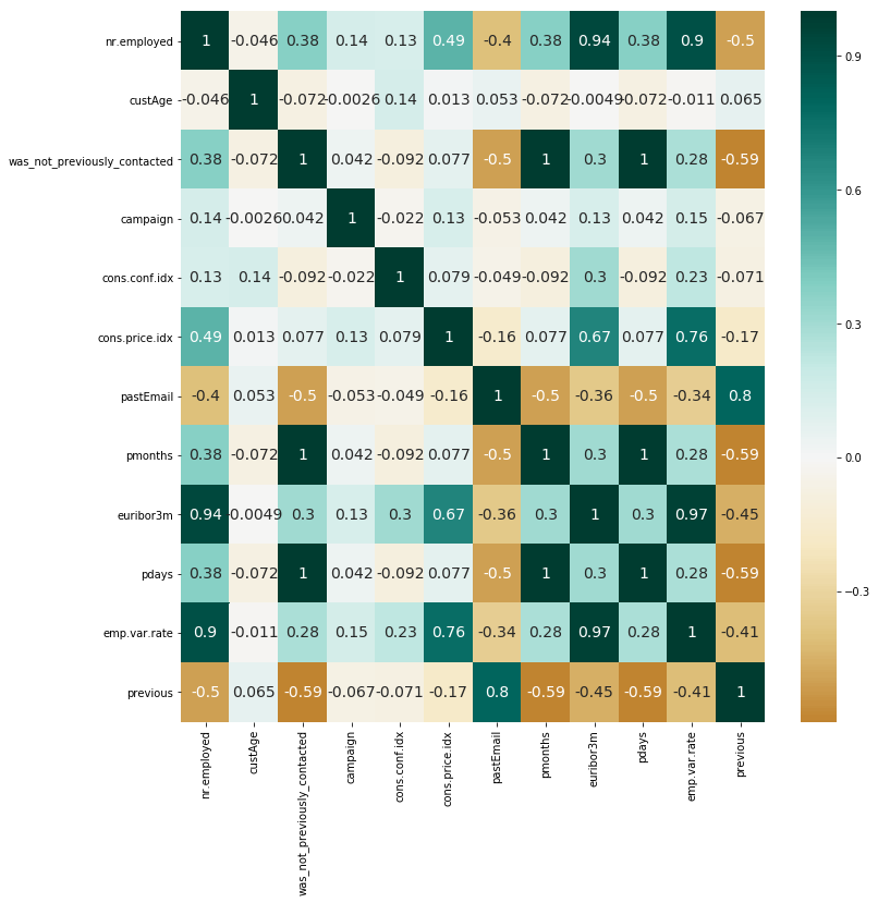
There is many correlation cases between features
Training the classifier
In this particular case, I have chosen to train our classifier using the LogisticRegression module from SciKit Learn, since it's a good starting point for a model, especially when our data is not too large.
To normalize the values, I use the StandardScaler, again from SciKit-Learn.
from sklearn.preprocessing import StandardScaler
scaler = StandardScaler()
x_train_scaled = scaler.fit_transform(x_train)
In the next line I look at the result of scaling. The first table of output shows the statistics for the original values. The second table shows the stats for the scaled values. Column 0 is Age and column 1 is KM.
print(pd.DataFrame(x_train).describe().round(2))
print(pd.DataFrame(x_train_scaled).describe().round(2))
            0        1        2        3        4        5        6        7   \
count  9938.00  9938.00  9938.00  9938.00  9938.00  9938.00  9938.00  9938.00
mean   5132.88    40.37     0.88     2.29   -40.31    93.48     0.55   881.81
std      87.36    10.77     0.32     2.26     5.34     0.63     1.55   321.44
min    4963.60    18.00     0.00     1.00   -50.80    92.20     0.00     0.00
25%    5076.20    33.03     1.00     1.00   -46.20    92.93     0.00   999.00
50%    5099.10    38.73     1.00     1.88   -41.80    93.44     0.00   999.00
75%    5228.10    44.04     1.00     2.87   -36.40    93.99     0.00   999.00
max    5228.10    94.00     1.00    40.00   -26.90    94.77    18.00   999.00

            8        9    ...          55       56       57       58       59  \
count  9938.00  9938.00   ...     9938.00  9938.00  9938.00  9938.00  9938.00
mean      2.91   882.51   ...        0.04     0.04     0.17     0.28     0.20
std       1.89   319.52   ...        0.18     0.19     0.35     0.42     0.37
min       0.63     0.00   ...        0.00     0.00     0.00     0.00     0.00
25%       1.25   999.00   ...        0.00     0.00     0.00     0.00     0.00
50%       1.47   999.00   ...        0.00     0.00     0.00     0.00     0.00
75%       4.96   999.00   ...        0.00     0.00     0.00     0.69     0.09
max       5.04   999.00   ...        1.00     1.00     1.00     1.00     1.00

            60       61       62       63       64
count  9938.00  9938.00  9938.00  9938.00  9938.00
mean      0.18     0.17     0.11     0.79     0.11
std       0.36     0.35     0.29     0.40     0.31
min       0.00     0.00     0.00     0.00     0.00
25%       0.00     0.00     0.00     1.00     0.00
50%       0.00     0.00     0.00     1.00     0.00
75%       0.00     0.00     0.00     1.00     0.00
max       1.00     1.00     1.00     1.00     1.00

[8 rows x 65 columns]
            0        1        2        3        4        5        6        7   \
count  9938.00  9938.00  9938.00  9938.00  9938.00  9938.00  9938.00  9938.00
mean     -0.00     0.00     0.00     0.00     0.00     0.00     0.00    -0.00
std       1.00     1.00     1.00     1.00     1.00     1.00     1.00     1.00
min      -1.94    -2.08    -2.74    -0.57    -1.97    -2.04    -0.35    -2.74
25%      -0.65    -0.68     0.36    -0.57    -1.10    -0.89    -0.35     0.36
50%      -0.39    -0.15     0.36    -0.18    -0.28    -0.06    -0.35     0.36
75%       1.09     0.34     0.36     0.26     0.73     0.81    -0.35     0.36
max       1.09     4.98     0.36    16.69     2.51     2.04    11.23     0.36

            8        9    ...          55       56       57       58       59  \
count  9938.00  9938.00   ...     9938.00  9938.00  9938.00  9938.00  9938.00
mean      0.00     0.00   ...       -0.00     0.00    -0.00     0.00     0.00
std       1.00     1.00   ...        1.00     1.00     1.00     1.00     1.00
min      -1.21    -2.76   ...       -0.23    -0.22    -0.49    -0.66    -0.53
25%      -0.88     0.36   ...       -0.23    -0.22    -0.49    -0.66    -0.53
50%      -0.76     0.36   ...       -0.23    -0.22    -0.49    -0.66    -0.53
75%       1.08     0.36   ...       -0.23    -0.22    -0.49     0.98    -0.29
max       1.13     0.36   ...        5.21     5.04     2.35     1.73     2.18

            60       61       62       63       64
count  9938.00  9938.00  9938.00  9938.00  9938.00
mean     -0.00     0.00     0.00     0.00    -0.00
std       1.00     1.00     1.00     1.00     1.00
min      -0.51    -0.49    -0.37    -1.96    -0.35
25%      -0.51    -0.49    -0.37     0.53    -0.35
50%      -0.51    -0.49    -0.37     0.53    -0.35
75%      -0.51    -0.49    -0.37     0.53    -0.35
max       2.27     2.37     3.05     0.53     2.91

[8 rows x 65 columns]
from sklearn import linear_model
# Create a linear model for Logistic Regression
clf = linear_model.LogisticRegression(C=1)

# we create an instance of Neighbours Classifier and fit the data.
clf.fit(x_train_scaled, y_train)
LogisticRegression(C=1, class_weight=None, dual=False, fit_intercept=True,
          intercept_scaling=1, max_iter=100, multi_class='warn',
          n_jobs=None, penalty='l2', random_state=None, solver='warn',
          tol=0.0001, verbose=0, warm_start=False)
from sklearn.metrics import accuracy_score
x_test_scaled = scaler.transform(x_test)
score = accuracy_score(y_test, clf.predict(x_test_scaled))
print("Model Accuracy: {}".format(score.round(3)))
Model Accuracy: 0.802


/home/mohcine/Software/anaconda2/lib/python2.7/site-packages/ipykernel_launcher.py:2: DataConversionWarning: Data with input dtype uint8, int64, float64 were all converted to float64 by StandardScaler.
from sklearn.metrics import recall_score
print 'test Results: Accuracy and recall'
print clf.score(x_test_scaled, y_test)
print recall_score(y_test, clf.predict(x_test_scaled))
print '\nTraining Results: Accuracy and recall'
print clf.score(x_train_scaled, y_train)
print recall_score(y_train, clf.predict(x_train_scaled))
test Results: Accuracy and recall
0.802049622437972
0.6465863453815262

Training Results: Accuracy and recall
0.7534715234453613
0.6914872207687663
Conclusion
-
The training results closely match the unseen test data results, which is exactly what I would want to see after putting a model into production.
-
80% accuracy looks good, but not too good classifying non responded customers (Recall). In statistics, recall is the number of correctly predicted “positives” divided by the total number of “positives”.
from sklearn.ensemble import RandomForestClassifier
clf_rf = RandomForestClassifier(n_estimators=25, random_state=12)
clf_rf.fit(x_train_scaled, y_train)
RandomForestClassifier(bootstrap=True, class_weight=None, criterion='gini',
            max_depth=None, max_features='auto', max_leaf_nodes=None,
            min_impurity_decrease=0.0, min_impurity_split=None,
            min_samples_leaf=1, min_samples_split=2,
            min_weight_fraction_leaf=0.0, n_estimators=25, n_jobs=None,
            oob_score=False, random_state=12, verbose=0, warm_start=False)
imp = pd.DataFrame(
        clf_rf.feature_importances_ ,
        columns = ['Importance'] ,
        index = list(num_cat_data)
    )
imp = imp.sort_values( [ 'Importance' ] , ascending = True )
#f1 = plt.figure()
f1, ax = plt.subplots(figsize=(12,12))
imp['Importance'].plot(kind='barh')
f1.show()
/home/mohcine/Software/anaconda2/lib/python2.7/site-packages/matplotlib/figure.py:457: UserWarning: matplotlib is currently using a non-GUI backend, so cannot show the figure
  "matplotlib is currently using a non-GUI backend, "
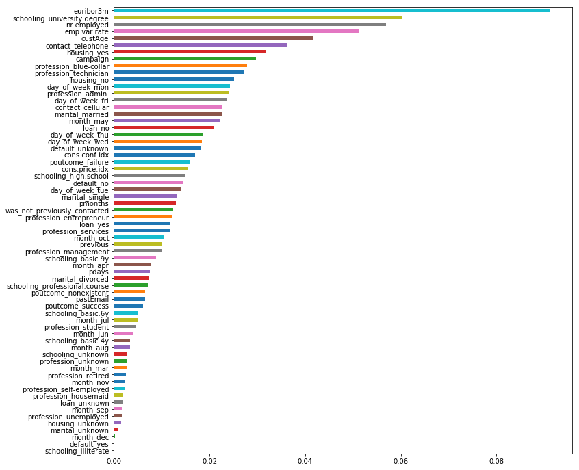
Conclusion:
I was expecting custAge, euribor3m, and schooling_university degree to be among the important features in predition
3- Building Prediction Model
import os
# Requirement in order to import xgboost
mingw_path = 'C:\\Program Files\\mingw-w64\\x86_64-6.1.0-posix-seh-rt_v5-rev0\\mingw64\\bin'
os.environ['PATH'] = mingw_path + ';' + os.environ['PATH']

#import all relevant libraries
import xgboost as xgb
from xgboost.sklearn import XGBClassifier
from xgboost import plot_importance
import pandas as pd
import numpy as np
import matplotlib.pyplot as plt
from sklearn.model_selection import GridSearchCV, StratifiedKFold
from sklearn.metrics import classification_report, confusion_matrix, precision_score, recall_score, roc_curve, auc
from scipy import interp

%matplotlib inline
# Define the class weight scale (a hyperparameter) as the ration of negative labels to positive labels.
# This instructs the classifier to address the class imbalance.
class_weight_scale = 1.*(y_train == 0).sum()/(y_train == 1).sum()
class_weight_scale
1.0
# Setting minimal required initial hyperparameters

param={
    'objective':'binary:logistic',
    'nthread':4,
    'scale_pos_weight':class_weight_scale,
    'seed' : 1
}
xgb1 = XGBClassifier()
xgb1.set_params(**param)
XGBClassifier(base_score=0.5, booster='gbtree', colsample_bylevel=1,
       colsample_bytree=1, gamma=0, learning_rate=0.1, max_delta_step=0,
       max_depth=3, min_child_weight=1, missing=None, n_estimators=100,
       n_jobs=1, nthread=4, objective='binary:logistic', random_state=0,
       reg_alpha=0, reg_lambda=1, scale_pos_weight=1.0, seed=1,
       silent=True, subsample=1)
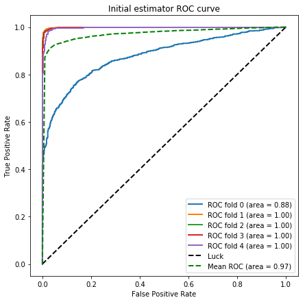
# Train initial classifier and analyze performace using K-fold cross-validation
K = 5
eval_size = int(np.round(1./K))
skf = StratifiedKFold(n_splits=K)

fig = plt.figure(figsize=(7,7))
mean_tpr = 0.0
mean_fpr = np.linspace(0, 1, 100)
lw = 2
i = 0
roc_aucs_xgb1 = []
for train_indices, test_indices in skf.split(x_train, y_train):
    X_train, Y_train = x_train[train_indices], y_train[train_indices]
    X_valid, y_valid = x_train[test_indices], y_train[test_indices]
    class_weight_scale = 1.*(y_train == 0).sum()/(y_train == 1).sum()
    print 'class weight scale : {}'.format(class_weight_scale)
    xgb1.set_params(**{'scale_pos_weight' : class_weight_scale})
    xgb1.fit(X_train,Y_train)
    xgb1_pred_prob = xgb1.predict_proba(X_valid)
    fpr, tpr, thresholds = roc_curve(y_valid, xgb1_pred_prob[:, 1])
    mean_tpr += interp(mean_fpr, fpr, tpr)
    mean_tpr[0] = 0.0
    roc_auc = auc(fpr, tpr)
    roc_aucs_xgb1.append(roc_auc)
    plt.plot(fpr, tpr, lw=2, label='ROC fold %d (area = %0.2f)' % (i, roc_auc))

    i += 1

plt.plot([0, 1], [0, 1], linestyle='--', lw=lw, color='k',
         label='Luck')

mean_tpr /= K
mean_tpr[-1] = 1.0
mean_auc = auc(mean_fpr, mean_tpr)
plt.plot(mean_fpr, mean_tpr, color='g', linestyle='--',
         label='Mean ROC (area = %0.2f)' % mean_auc, lw=lw)

plt.xlim([-0.05, 1.05])
plt.ylim([-0.05, 1.05])
plt.xlabel('False Positive Rate')
plt.ylabel('True Positive Rate')
plt.title('Initial estimator ROC curve')
plt.legend(loc="lower right")

fig.savefig('figures/initial_ROC.png')
[1129 1130 1131 ... 9935 9936 9937]
class weight scale : 1.0
[   0    1    2 ... 9935 9936 9937]
class weight scale : 1.0
[   0    1    2 ... 9935 9936 9937]
class weight scale : 1.0
[   0    1    2 ... 9935 9936 9937]
class weight scale : 1.0
[   0    1    2 ... 8942 8943 8944]
class weight scale : 1.0
Regularization of the Prediction Model
# Option to perform hyperparameter optimization. Otherwise loads pre-defined xgb_opt params
optimize = True
X_train = x_train
y_train = y_train

if optimize:

    param_test0 = {
     'n_estimators':range(50,250,10)
    }
    print 'performing hyperparamter optimization step 0'
    gsearch0 = GridSearchCV(estimator = xgb1, param_grid = param_test0, scoring='roc_auc',n_jobs=4,iid=False, cv=5)
    gsearch0.fit(X_train,y_train)
    print gsearch0.best_params_, gsearch0.best_score_

    param_test1 = {
     'max_depth':range(1,10),
     'min_child_weight':range(1,10)
    }
    print 'performing hyperparamter optimization step 1'
    gsearch1 = GridSearchCV(estimator = gsearch0.best_estimator_,
     param_grid = param_test1, scoring='roc_auc',n_jobs=4,iid=False, cv=5)
    gsearch1.fit(X_train,y_train)
    print gsearch1.best_params_, gsearch1.best_score_

    max_d = gsearch1.best_params_['max_depth']
    min_c = gsearch1.best_params_['min_child_weight']

    param_test2 = {
     'gamma':[i/10. for i in range(0,5)]
    }
    print 'performing hyperparamter optimization step 2'
    gsearch2 = GridSearchCV(estimator = gsearch1.best_estimator_,
     param_grid = param_test2, scoring='roc_auc',n_jobs=4,iid=False, cv=5)
    gsearch2.fit(X_train,y_train)
    print gsearch2.best_params_, gsearch2.best_score_

    param_test3 = {
        'subsample':[i/10.0 for i in range(1,10)],
        'colsample_bytree':[i/10.0 for i in range(1,10)]
    }
    print 'performing hyperparamter optimization step 3'
    gsearch3 = GridSearchCV(estimator = gsearch2.best_estimator_,
     param_grid = param_test3, scoring='roc_auc',n_jobs=4,iid=False, cv=5)
    gsearch3.fit(X_train,y_train)
    print gsearch3.best_params_, gsearch3.best_score_

    param_test4 = {
        'reg_alpha':[0, 1e-5, 1e-3, 0.1, 10]
    }
    print 'performing hyperparamter optimization step 4'
    gsearch4 = GridSearchCV(estimator = gsearch3.best_estimator_,
     param_grid = param_test4, scoring='roc_auc',n_jobs=4,iid=False, cv=5)
    gsearch4.fit(X_train,y_train)
    print gsearch4.best_params_, gsearch4.best_score_

    alpha = gsearch4.best_params_['reg_alpha']
    if alpha != 0:
        param_test4b = {
            'reg_alpha':[0.1*alpha, 0.25*alpha, 0.5*alpha, alpha, 2.5*alpha, 5*alpha, 10*alpha]
        }
        print 'performing hyperparamter optimization step 4b'
        gsearch4b = GridSearchCV(estimator = gsearch4.best_estimator_,
         param_grid = param_test4b, scoring='roc_auc',n_jobs=4,iid=False, cv=5)
        gsearch4b.fit(X_train,y_train)
        print gsearch4b.best_params_, gsearch4.best_score_
        print '\nParameter optimization finished!'
        xgb_opt = gsearch4b.best_estimator_
        xgb_opt
    else:
        xgb_opt = gsearch4.best_estimator_
        xgb_opt
else:
    # Pre-optimized settings
    xgb_opt = XGBClassifier(base_score=0.5, colsample_bylevel=1, colsample_bytree=0.7,
       gamma=0.1, learning_rate=0.1, max_delta_step=0, max_depth=3,
       min_child_weight=5, missing=None, n_estimators=70, nthread=4,
       objective='binary:logistic', reg_alpha=25.0, reg_lambda=1,
       scale_pos_weight=7.0909090909090908, seed=1, silent=True,
       subsample=0.6)

print xgb_opt
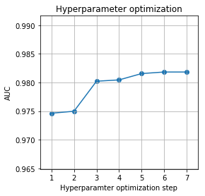
performing hyperparamter optimization step 0
{'n_estimators': 110} 0.9749764110312029
performing hyperparamter optimization step 1
{'max_depth': 9, 'min_child_weight': 1} 0.9802166944977622
performing hyperparamter optimization step 2
{'gamma': 0.1} 0.980447807952243
performing hyperparamter optimization step 3
{'subsample': 0.4, 'colsample_bytree': 0.9} 0.9815532764983201
performing hyperparamter optimization step 4
{'reg_alpha': 0.001} 0.9818254583224896
performing hyperparamter optimization step 4b
{'reg_alpha': 0.001} 0.9818254583224896

Parameter optimization finished!
XGBClassifier(base_score=0.5, booster='gbtree', colsample_bylevel=1,
       colsample_bytree=0.9, gamma=0.1, learning_rate=0.1,
       max_delta_step=0, max_depth=9, min_child_weight=1, missing=None,
       n_estimators=110, n_jobs=1, nthread=4, objective='binary:logistic',
       random_state=0, reg_alpha=0.001, reg_lambda=1, scale_pos_weight=1.0,
       seed=1, silent=True, subsample=0.4)
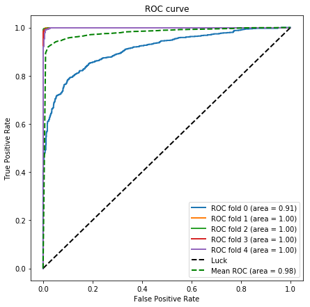
K-fold cross-validation
K = 5
eval_size = int(np.round(1./K))
skf = StratifiedKFold(n_splits=K)


fig = plt.figure(figsize=(7,7))
mean_tpr = 0.0
mean_fpr = np.linspace(0, 1, 100)
lw = 2
i = 0
roc_aucs_xgbopt = []
for train_indices, test_indices in skf.split(x_train, y_train):
    X_train, Y_train = x_train[train_indices], y_train[train_indices]
    X_valid, y_valid = x_train[test_indices], y_train[test_indices]
    class_weight_scale = 1.*(y_train == 0).sum()/(y_train == 1).sum()
    print 'class weight scale : {}'.format(class_weight_scale)
    xgb_opt.set_params(**{'scale_pos_weight' : class_weight_scale})
    xgb_opt.fit(X_train,Y_train)
    xgb_opt_pred_prob = xgb_opt.predict_proba(X_valid)
    fpr, tpr, thresholds = roc_curve(y_valid, xgb_opt_pred_prob[:, 1])
    mean_tpr += interp(mean_fpr, fpr, tpr)
    mean_tpr[0] = 0.0
    roc_auc = auc(fpr, tpr)
    roc_aucs_xgbopt.append(roc_auc)
    plt.plot(fpr, tpr, lw=2, label='ROC fold %d (area = %0.2f)' % (i, roc_auc))

    i += 1

plt.plot([0, 1], [0, 1], linestyle='--', lw=lw, color='k',
         label='Luck')

mean_tpr /= K
mean_tpr[-1] = 1.0
mean_auc = auc(mean_fpr, mean_tpr)
plt.plot(mean_fpr, mean_tpr, color='g', linestyle='--',
         label='Mean ROC (area = %0.2f)' % mean_auc, lw=lw)

plt.xlim([-0.05, 1.05])
plt.ylim([-0.05, 1.05])
plt.xlabel('False Positive Rate')
plt.ylabel('True Positive Rate')
plt.title('ROC curve')
plt.legend(loc="lower right")

fig.savefig('figures/ROC.png')
class weight scale : 1.0
class weight scale : 1.0
class weight scale : 1.0
class weight scale : 1.0
class weight scale : 1.0
if optimize:

    aucs = [np.mean(roc_aucs_xgb1),
            gsearch0.best_score_,
            gsearch1.best_score_,
            gsearch2.best_score_,
            gsearch3.best_score_,
            gsearch4.best_score_,
            np.mean(roc_aucs_xgbopt)]

    fig = plt.figure(figsize=(4,4))
    plt.scatter(np.arange(1,len(aucs)+1), aucs)
    plt.plot(np.arange(1,len(aucs)+1), aucs)
    plt.xlim([0.5, len(aucs)+0.5])
    plt.ylim([0.99*aucs[0], 1.01*aucs[-1]])
    plt.xlabel('Hyperparamter optimization step')
    plt.ylabel('AUC')
    plt.title('Hyperparameter optimization')
    plt.grid()
    fig.savefig('figures/optimization.png')
precision recall f1-score of testing set
print classification_report(y_true = y_test.values, y_pred = xgb_opt.predict(x_test.values))
              precision    recall  f1-score   support

           0       0.90      0.97      0.93      1605
           1       0.60      0.30      0.40       249

   micro avg       0.88      0.88      0.88      1854
   macro avg       0.75      0.64      0.67      1854
weighted avg       0.86      0.88      0.86      1854
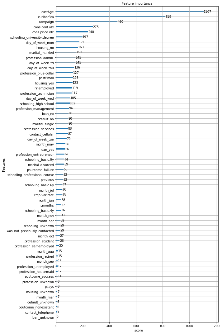
Features Importance
xgb_opt.get_booster().feature_names = list(x_test)
def my_plot_importance(booster, figsize, **kwargs):
    from matplotlib import pyplot as plt
    from xgboost import plot_importance
    fig, ax = plt.subplots(1,1,figsize=(figsize))
    plot_importance(booster=booster, ax=ax, **kwargs)
    for item in ([ax.title, ax.xaxis.label, ax.yaxis.label,] +
ax.get_xticklabels() + ax.get_yticklabels()):
        item.set_fontsize(10)
    plt.tight_layout()
    fig.savefig('figures/Feature_importance.png')

my_plot_importance(xgb_opt, (10,15))
comments powered by Disqus