Assets Management and energy demand forecasting using Matrix Profile

The code of this article is available at: https://github.com/mohcinemadkour/Matrix-Profile-for-Regime-Detection-in-Time-Series-Data/tree/master

Today’s companies hold enormous value in the form of equipment and plants. Research suggests that on average, 5 to 15 % of a manufacturing company’s global asset base is idle, with most not having good visibility of these underutilized assets. In pharmaceutical industry for example, finding and repurposing under-utilized assets is seen to deliver the highest value and proven to avoid $ Millions of capital expenditures.

Recent advances in time series classification and forecasting such as Prophet, Matrix Profile, RNN brought sophisticated tools to the support of the visibility and control of energy consumption at the device level. For example, identifying pattern of usage episodes overlaid on asset energy consumption can help to compare usage periods by location, type of equipment, and even individual device. However in real-life problem domain every situation is different and therefore using frequency domain or statistically modeling techniques, for example, to find patterns of energy consumption will require domain specific knowledge and to have labels on data which sometimes can bottleneck the motif search process. In this article I show a new technique that’s based on matrix profile to detect episodes of electricity usage and return the timestamps at which each episode stars and stops.

Data set and problem description

In this example we show energy consumption data from a pharmaceutical equipment over the course of a typical 24-hour day. Power consumption is measured in watts. The behavior of the device being measured is fairly typical: during episodes of active usage, power consumption quickly increases from an “idle” or background level of consumption, and then returns to idle power draw after usage ceases. Power consumption is noisy and variable in general. It is also fairly common for the “background” consumption of equipment to be variable over time, noisy, and to change such that you cannot rely on a single measurement or value.

Calculation of Matrix Profile

The Matrix Profile is a relatively new data structure for time series analysis developed by Eamonn Keogh at the University of California Riverside and Abdullah Mueen at the University of New Mexico []. Some of the advantages of using the Matrix Profile is that it is domain agnostic, fast, provides an exact solution (approximate when desired) and only requires a single parameter. The algorithms that compute the Matrix Profile use a sliding window approach. With a window size of m, the algorithm: - Computes the distances for the windowed sub-sequence against the entire time series - Sets an exclusion zone to ignore trivial matches - Updates the distance profile with the minimal values - Sets the first nearest-neighbor index The distance calculations outlined above occur n-m + 1 times; where n is the length of the time series and m is the window size. Since the sub-sequences are pulled from the time series itself, an exclusion zone is required to prevent trivial matches. For example, a snippet matching itself or a snippet very close to itself is considered a trivial match. The exclusion zone is simply half of the window size (m) both before and after the current window index. The values at these indices are ignored when computing the minimum distance and the nearest-neighbor index. A visualization showing the computation of a distance profile starting at the second window is shown below.

The second window of values, X2 through X5, slides across the time series computing the dot product for each sub-sequence. Once all of the dot products are computed, the exclusion zone is applied to the distances and the minimum distance is stored in the Matrix Profile. Throwing away the extra distances and only keeping the minimum distance reduces the space complexity to 0(n).

Motif (and Anomaly) Definitions

A motif is a repeated pattern in a time series and a discord is an anomaly. With the Matrix Profile computed, it is simple to find the top-K number of motifs or discords. The Matrix Profile stores the distances in Euclidean space meaning that a distance close to 0 is most similar to another sub-sequence in the time series and a distance far away from 0, say 100, is unlike any other sub-sequence. Extracting the lowest distances gives the motifs and the largest distances gives the discords.

def calc_mp_cac(df,m):
    warnings.filterwarnings('ignore')
    pattern = df.power.values
    mp = matrixProfile.stomp(pattern,m)
    # Bonus: calculate the corrected arc curve (CAC) to do semantic segmantation.
    cac = fluss.fluss(mp[1], m)
    #Append np.nan to Matrix profile to enable plotting against raw data
    mp_adj = np.append(mp[0],np.zeros(m-1)+np.nan)
    #Plot the signal data
    fig, (ax1, ax2, ax3) = plt.subplots(3,1,sharex=True,figsize=(20,10))
    ax1.plot(np.arange(len(pattern)),pattern, label="Power Consumption Data")
    ax1.set_ylabel('Signal', size=22)
    #Plot the Matrix Profile
    ax2.plot(np.arange(len(mp_adj)),mp_adj, label="Matrix Profile", color='red')
    ax2.set_ylabel('Matrix Profile', size=22)
    ax2.set_xlabel("Sequence window={}".format(m), size=22)
    #Plot the CAC
    ax3.plot(np.arange(len(cac)),cac, label="CAC", color='green')
    ax3.set_ylabel('CAC', size=22)
    ax3.set_xlabel("Sequence window={}".format(m), size=22)
    return mp

def plot_mp_cac(df,m, feature,mp):
    warnings.filterwarnings('ignore')
    pattern = df[feature].values
    # Bonus: calculate the corrected arc curve (CAC) to do semantic segmantation.
    cac = fluss.fluss(mp[1], m)

    #Append np.nan to Matrix profile to enable plotting against raw data
    mp_adj = np.append(mp[0],np.zeros(m-1)+np.nan)

    #Plot the signal data
    fig, (ax1, ax2, ax3) = plt.subplots(3,1,sharex=True,figsize=(20,10))
    ax1.plot(np.arange(len(pattern)),pattern, label="Power Consumption Data")
    ax1.set_ylabel('Signal', size=22)

    #Plot the Matrix Profile
    ax2.plot(np.arange(len(mp_adj)),mp_adj, label="Matrix Profile", color='red')
    ax2.set_ylabel('Matrix Profile', size=22)
    ax2.set_xlabel("Sequence window={}".format(m), size=22)

    #Plot the CAC
    ax3.plot(np.arange(len(cac)),cac, label="CAC", color='green')
    ax3.set_ylabel('CAC', size=22)
    ax3.set_xlabel("Sequence window={}".format(m), size=22)
    return mp

def plot_signal_mp(df,m, feature,mp):
    warnings.filterwarnings('ignore')
    pattern = df[feature].values

    #Append np.nan to Matrix profile to enable plotting against raw data
    mp_adj = np.append(mp[0],np.zeros(m-1)+np.nan)

    #Plot the signal data
    fig, (ax1, ax2) = plt.subplots(2,1,sharex=True,figsize=(20,10))
    ax1.plot(np.arange(len(pattern)),pattern, label="Power Consumption Data")
    ax1.set_ylabel('Signal', size=22)

    #Plot the Matrix Profile
    ax2.plot(np.arange(len(mp_adj)),mp_adj, label="Matrix Profile", color='red')
    ax2.set_ylabel('Matrix Profile', size=22)
    ax2.set_xlabel("Sequence window={}".format(m), size=22)

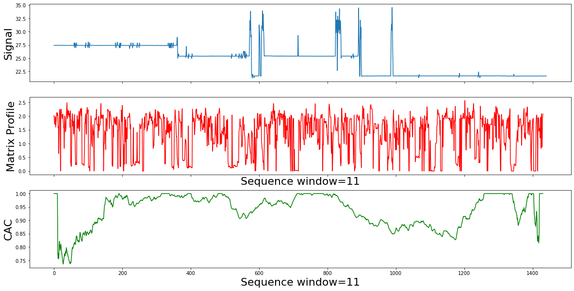
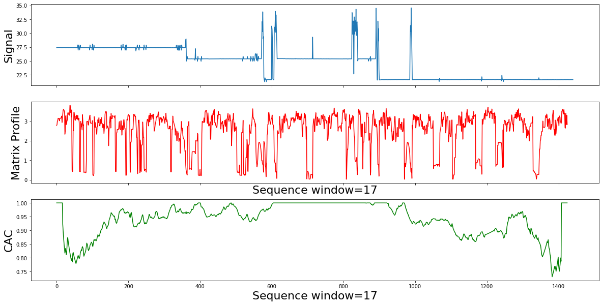
mp=calc_mp_cac(df,11)

Summary:

Interpretation of the matrix profile (mp) plot form the mp plot, there are many items of note:

• The choice of the subsequence lengh can be made visually, from the pattern examples, we are only interested in small local subsequences, of length ~ 11 min
• The relatively low values implies that the subsequence in the original time series must have (at least one) relatively similar subsequence elsewhere in the time series data (such regions are “motifs” or reoccurring patterns)
• Repeated patterns in the data (or "motifs") lead to low Matrix Profile values: From the data it looks that we dont have reapeted motifts throughout the time Where we see relatively high values , we know that the subsequence in the original time series must be unique in its shape (such areas are “discords” )
• The Matrix Profile value jumps at each phase change. High Matrix Profile values are associated with "discords": time series behavior that hasn't been observed before: From the mp it looks we have many jumps because the time series data keeps fluctuating but there is no standalone top or local tops which means there it is no Discord or Anomay
• The conclusion is that the data is noisy and domain knowledge informtion is missing

Matrix Profile Segmentation

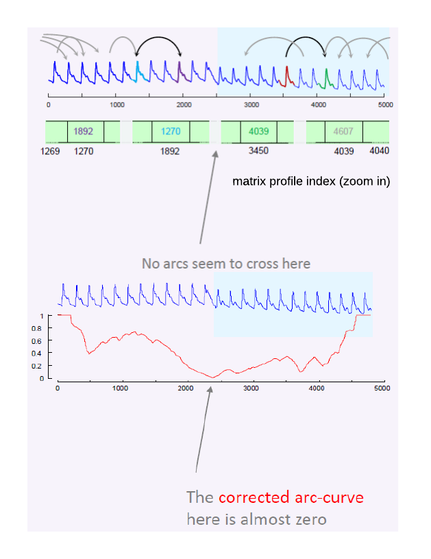
The Matrix Profile allows a simple algorithm, FLUSS/FLOSS, for time series segmentation.The ideas of segmentation comes form the Matrix Profile Index which has pointers ( arrows , arcs ) that point to the nearest neighbor of each subsequence. If we have a change of behavior, for exampe active to idle , we should expect very few arrows to span that change of behavior (See the arrows in the bellow picture). In the matrixprofile-ts python library, the fluss function is implemented in the fluss sub-module, and it outputs the corrected arc curve

Notes:

• Most active subsequences will point to another active subsequence
• Most "idle" subsequences will point to another "idle" subsequence
• Rarely, if ever, will an "idle" point to an "active"

So, if we slide across the Matrix Profile Index , and count how many arrows cross each particular point, we expect to find few that span the change of behavior. As we can see in the example used in the corrected arc curve (CAC) bellow, The CAC minimizes in the right place. The CAC has a single parameter, the subsequence length m .Lets change it by an order of magnitude, and see how the results will change.

for m in [11,14,17]:
    calc_mp_cac(df,m)

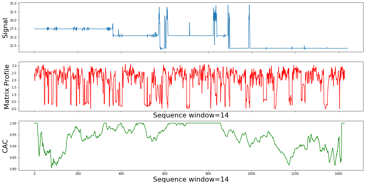
Summury

• The segmentation result sounds mathematically correct, but not what we expect for the active power domain.
• The true motifs are still “swamped” by more frequent, but meaningless patterns, like idle patterns.
• The solutions is to correctly incorporates the contextual weights of noise and active consumption in our use case.
• By correcting the MP to bias away from idle motifs, we can discover meaningful power active usage motifs.
• In the next step we will supress the 'motifs' that we know are representing idle or noise.

Domain specific annotation vector : Corrected Matrix Profile

The annotation vector( AV ) is a time series consisting of real valued numbers between [0 1]. A lower value indicates the subsequence starting at that index is less desirable, and therefore should be biased against . Conversely, higher values mean the corresponding subsequences should be favored for the potential motif pool.

from matrixprofile.utils import apply_av
def av_power_consumption(df, m, feature, height, disp=True):
    pattern = df[feature].values
    mp = matrixProfile.stomp(pattern,m)
    av=np.zeros(np.shape(mp)[1])
    ind=0
    max=np.max(df[feature])
    for i in df.index:
        if(df.loc[i,"power"]>max-height):
            av[ind]=1
        ind=ind+1
    mp_corrected=apply_av(mp,av)
    if (disp==True):
        plot_signal_mp(df,m, "power",mp_corrected)
    return mp_corrected
mp_corrected=av_power_consumption(df, 12, "power", 5)

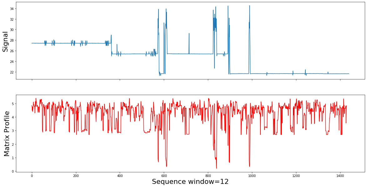
Summury

After adding the domain knowledge information( represented by the AV), the Corrected matrix profile is capable of detecting the consumption motifs by showing them as the low values

Motif Search

After finding some relatively low values (almost 0) in the mp, lets find out the different motifs existing in our data

def plot_motifs(mtfs, labels, ax):
    colori = 0
    colors = 'rgbcm'
    for ms,l in zip(mtfs,labels):
        c =colors[colori % len(colors)]
        starts = list(ms)
        ends = [min(s + m,len(pattern)-1) for s in starts]
        ax.plot(starts, pattern[starts],  c +'o',  label=l)
        ax.plot(ends, pattern[ends],  c +'o', markerfacecolor='none')
        for nn in ms:
            ax.plot(range(nn,nn+m),pattern[nn:nn+m], c , linewidth=2)
        colori += 1
    ax.plot(pattern, 'k', linewidth=1, label="data")
    ax.legend()
mp_corrected=av_power_consumption(df, 12, "power", 5, disp="False")
mtfs ,motif_d  = motifs.motifs(pattern, mp_corrected, max_motifs=3)

def plot_signal_cmp_motifs(df, feature,m,mp_corrected ):
    warnings.filterwarnings('ignore')
    pattern = df[feature].values
    #Append np.nan to Matrix profile to enable plotting against raw data
    mp_adj = np.append(mp_corrected[0],np.zeros(m-1)+np.nan)

    #Plot the signal data
    fig, (ax1, ax2, ax3) = plt.subplots(3,1,sharex=True,figsize=(20,10))
    ax1.plot(np.arange(len(pattern)),pattern, label="power Data")
    ax1.set_ylabel('Signal', size=22)

    #Plot the corrected Matrix Profile
    ax2.plot(np.arange(len(mp_adj)),mp_adj, label="Corrected Matrix Profile", color='red')
    ax2.set_ylabel('Corrected Matrix Profile', size=22)

    #Plot the Motifs
    plot_motifs(mtfs, [f"{md:.3f}" for md in motif_d], ax3)
    ax3.set_ylabel('Motifs', size=22)
    #plt.xlim((0,100))
    plt.show()
plot_signal_cmp_motifs(df, "power",11,mp_corrected )

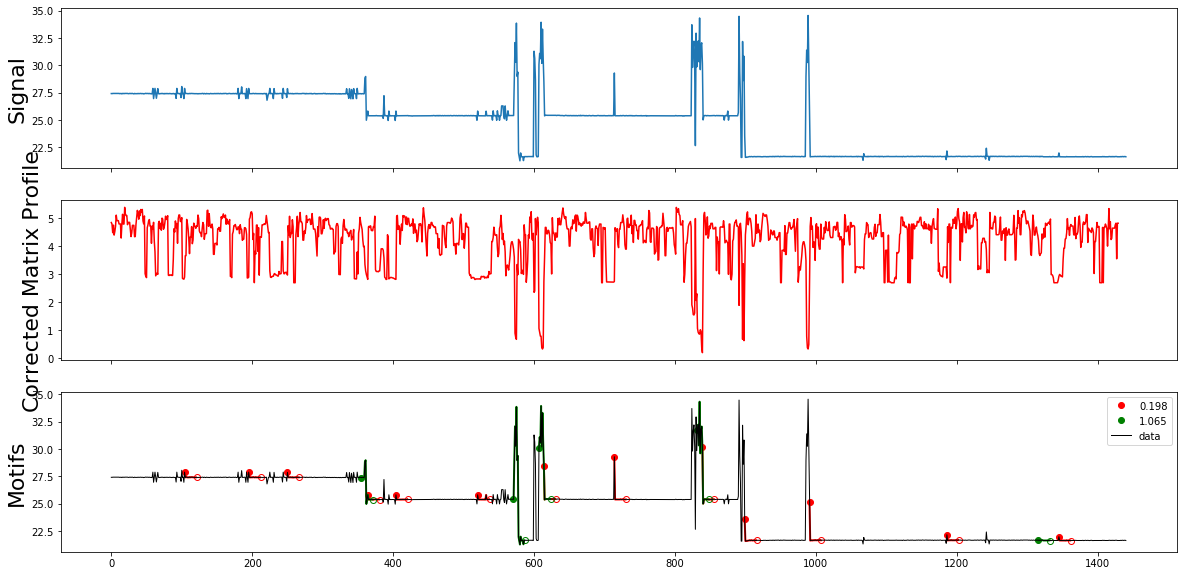
Summury

The motifs.motifs function founds some consumption patterns in the data as well as some noise motifs, we will try to tune the motif search in order to discover consumption motifs only

Motifs Discovery

The motifs.motifs function admits the following parametres and return

Parameters

• max_motifs: stop finding new motifs once we have max_motifs
• radius: For each motif found, find neighbors that are within radius*motif_mp of the first.
• n_neighbors: number of neighbors from the first to find. If it is None, find all.
• ex_zone: minimum distance between indices for after each subsequence is identified. Defaults to m/2 where m is the subsequence length. If ex_zone = 0, only the found index is exclude, if ex_zone = 1 then if idx is found as a motif idx-1, idx, idx+1 are excluded.

Returns The function returns a tuple (top_motifs, distances) which are lists of the same length.

• top_motifs: This is a list of the indices found for each motif. The first index is the nth motif followed by all nearest neighbors found sorted by distances.
• distances: Minimum Matrix profile value for each motif set. More detail about the algortihm implemented by this function can be found here: https://www.cs.ucr.edu/~eamonn/guided-motif-KDD17-new-format-10-pages-v005.pdf

Experimenetation

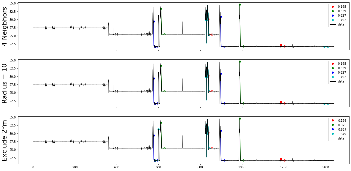
In this step we experimente different values of max_motifs, radius, n_neighbors, and ex_zone, and use motifs plots visualization to find the best parametres set that distiguish the consumption motifs

fig, (ax1, ax2, ax3) = plt.subplots(3,1,sharex=True,figsize=(20,10))


mtfs ,motif_d  = motifs.motifs(pattern, mp_corrected, max_motifs=5, n_neighbors=None, radius=0)
plot_motifs(mtfs, [f"{md:.3f}" for md in motif_d], ax1)
ax1.set_ylabel('4 Neigbhors', size=22)
print(mtfs)

#mtfs ,motif_d  = motifs.motifs(pattern, mp, max_motifs=5, radius=10)
mtfs ,motif_d  = motifs.motifs(pattern, mp_corrected, max_motifs=5, n_neighbors=0, radius=0)
plot_motifs(mtfs, [f"{md:.3f}" for md in motif_d], ax2)
ax2.set_ylabel('Radius = 10', size=22)
print(mtfs)

#mtfs ,motif_d  = motifs.motifs(pattern, mp, max_motifs=3, ex_zone=2)
mtfs ,motif_d  = motifs.motifs(pattern, mp_corrected, max_motifs=5, n_neighbors=None, radius=0,  ex_zone=5)
plot_motifs(mtfs, [f"{md:.3f}" for md in motif_d], ax3)
ax3.set_ylabel('Exclude 2*m', size=22)
plt.show()
print(mtfs)
#### Results:
[[839, 1186], [612, 989], [577, 898], [825, 1394]]
[[839, 1186], [612, 989], [577, 898], [825, 1394]]

Periods of active power consumptions

df.loc[(df.index>=839) & (df.index<=839+11)]
df.loc[(df.index>=1186) & (df.index<=1186+11)]
df.loc[(df.index>=612) & (df.index<=612+11)]
df.loc[(df.index>=989) & (df.index<=989+11)]
df.loc[(df.index>=577) & (df.index<=577+11)]    
df.loc[(df.index>=898) & (df.index<=898+11)]
df.loc[(df.index>=583) & (df.index<=583+11)]
df.loc[(df.index>=827) & (df.index<=827+11)]

General Conclusion

• By correcting the matrix profile with an AV based on the active power consumptions peaks measure, we were able to discover the true motifs
• After fine tuning the parametres of motifs.motifs, we were able to differtiate different motifs existing in the data.
• Visually we have one false positive : the red motif in the right, which we refere to noise. We can improve the result by adding a noise fiter on the found motifs.